Plotting Vector Data

In the last article we took a normal DataFrame containing mountain peaks and turned it into GeoDataFrame. We had the locations and the point geometries. But a bunch of points on their own doesn’t really tell us much.

In actual GIS work, we usually work with multiple layers of spatial data together. We might have points representing locations, lines representing roads and polygons representing things like countries, buildings etc.

So in this article, we will bring in another vector layer containing US boundaries and plot our mountain peaks on top of it. It will start to look a little more like actual GIS.

Getting the boundary data

In the previous article, we were working with points, this time we need some polygon data. A state boundary represents an area, so representing it as a Point wouldn’t make much sense. So instead each state will have a Polygon geometry representing it’s boundary.

For this we will use US state boundary data from the US Census Bureau’s Cartographic Boundary Files. This data is free to use and already follows EPSG:4326, which is the same CRS we used for our mountain peaks.

Download the shape file and place it inside your directory. Here is the link US State Boundary Files

Loading the boundary data

Let us load the file using GeoPandas :

import geopandas as gpd

states = gpd.read_file("https://cdn.jsdelivr.net/gh/anidotdev/us-census-shapefiles@main/cb_2023_us_state_20m.zip")
states.head()

OUTPUT

In the previous article, we manually created a Pandas DataFrame, converted the latitude and longitude into Point geometries, and then created a GeoDataFrame from it.

This time, things are a little different. The Shapefile already contains spatial data, so we can use read_file() to directly load it into a GeoDataFrame. The geometry column is already there. If you look at the geometry column, you will notice that these geometries are not Points like our mountain peaks instead they are polygons.

Each row represents the boundary of a state as a geometry and some geometries can contain multiple parts, which is represented as MultiPolygon in GeoPandas.

Filtering the states that we need

The full dataset contains all US states and some territories, but we don’t need all of that. Our mountain peaks are located in North Carolina, Tennessee and Virginia, so let’s only keep those states only:

target_states = ["North Carolina", "Tennessee", "Virginia"]

states_subset = states[states["NAME"].isin(target_states)]
states_subset

OUTPUT

If you have used Pandas before then this should look somewhat familiar, all we are doing is that we are just filtering rows based on the values in the NAME column. This is one of the nice things about GeoPandas that regular Pandas stuff works exactly as they was you’d expect. Now we have a smaller GeoDataFrame containing only the three states we actually need.

Bringing back our mountain peaks

Now let’s create our peaks GeoDataFrame again. If you came here from the previous article, you’ve already seen this part, but I’m adding it again so this article can also make sense on its own.

import pandas as pd

data = {
    "Peak Name": ["Mount Mitchell", "Clingmans Dome", "Mount Craig", "Mount Guyot", "McAfee Knob", "Adams Mountain"],
    "State/Province": ["North Carolina", "Tennessee", "North Carolina", "Tennessee/NC", "Virginia", "North Carolina"],
    "Elevation (m)": [2037, 2025, 2032, 2020, 974, 759],
    "Latitude": [35.7648, 35.5628, 35.7728, 35.6931, 37.3806, 35.9311],
    "Longitude": [-82.2652, -83.4980, -82.2653, -83.2417, -80.0367, -81.7244]
}

df = pd.DataFrame(data)

geometry = gpd.points_from_xy(df["Longitude"],df["Latitude"])

gdf = gpd.GeoDataFrame(df, geometry=geometry, crs="EPSG:4326")

Now we have two separate GeoDataFrames.

states_subset contains Polygon geometries representing state boundaries. gdf contains Point geometries representing mountain peaks. And both datasets use the same EPSG:4326. That means both layers are using the same CRS, so GeoPandas can easily place them relative to each other.

If you have different CRS then you could have points appearing in completely different locations, we will properly get into that in the next article, for now just remember that if you’re working with multiple spatial layers, checking their CRS is important.

Plotting both layers together

Now we will build the actual map, for that we will use folium, which is a python package to create interactive maps..

import folium

# Creating the the base map
m = folium.Map(
    location=[36.5, -81.8],
    zoom_start=6
)

# Adding state boundaries from the states_subset
folium.GeoJson(
    states_subset,
    name="State Boundaries",
    style_function=lambda feature: {
        "fillColor": "lightgrey",
        "color": "black",
        "weight": 1,
        "fillOpacity": 0.5,
    }
).add_to(m)

# Adding mountain peaks from the gdf GeoDataFrame
for _, row in gdf.iterrows():
    folium.CircleMarker(
        location=[row.geometry.y, row.geometry.x],
        radius=6,
        color="red",
        fill=True,
        fill_color="red",
        popup=row["Peak Name"]
    ).add_to(m)

# Finally displaying the map
m

OUTPUT

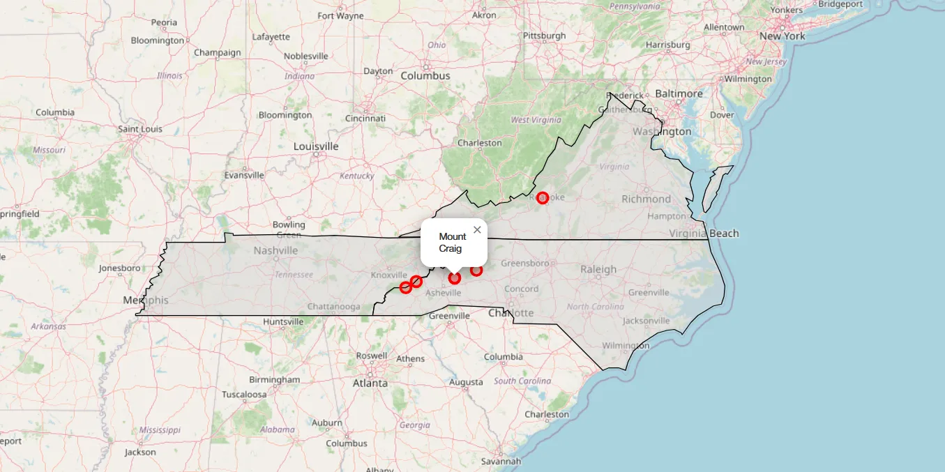
The important part here is that we’re adding both layers to the same Folium map object, m.

First, we add the state boundaries using folium.GeoJson(). This takes our Polygon data and adds it as a layer on the map. Then, we loop through the mountain peaks and add each one as a CircleMarker. Since each row in our GeoDataFrame contains a Point geometry, we can use its coordinates to place the marker at the correct location.

So now we have two different vector data, one is Point and the other is Polygon, which are displayed together on the same interactive map. This is a pretty basic example but as I learn more complex things myself, I will surely document more of it in my articles of GIS in the future.

That is it for this one… Happy Learning :D